Building your AI Ecosystem Part I: Data Architecture, Pipelines, and Dimensional Modelling

Introduction

In this article, we’ll give a broad overview of an architecture focused on data lakes and warehouses as well as a data orchestrator to perform some data integration and data modelling tasks. We will take a look at some distributed computing concepts as dimensional modelling, in hopes of giving an overview as to what it takes to build a data architecture that could fit your organization’s needs. This post (and series) is targeted at an audience with some technical background that has an interest at gaining a higher-level view of a data initiatives.

Suppose you’re the director for data initatives at a retail company. After discussing some interesting use cases with stakeholders, setting up the roadmap etc., you find yourself in front of the first technical task: designing the data architecture. To do that, let’s first investigate the data we could be utilizing / working with.

Understanding Data Sources

We have some internal data that employees make use of when understanding internal procedures and guidelines. They’re in the form of pdfs within a fileserver, such as FTP and SFTP. r data scientists that want to build an LLM. Our data scientists also want access to customer transactions data in order to build models that would help forecast their lifetime value and churn risk in order to prioritize the marketing team’s targeting initiatives.

While the DSs can gain access to the FTP and MongoDB servers, this adds an extra layers of security risk; the IT team is better off giving access to a centralized area to increase control while helping the DSs navigate the company’s data more accessibly.

To simplify the FTP server, we created a simple Python Flask Server that will serve our files. We’ll initially populate it by using the script under scripts/online_data_to_ftp_and_mongodb.py, which, like the name suggest, we also populate our MongoDB database; here’s a sample of the HR procedure:

And a sample of the MongoDB database’s data:

{
    _id: ObjectId('6634ed99e4cf3b4b5d6076d5'),
    InvoiceNo: '536365',
    StockCode: '85123A',
    Description: 'WHITE HANGING HEART T-LIGHT HOLDER',
    Quantity: 6,
    InvoiceDate: '12/1/2010 8:26',
    UnitPrice: 2.55,
    CustomerID: 17850,
    Country: 'United Kingdom'
}

You can find the instructions on how to setup the project in the README.md file of the project.

Building the Data Lake

After we populate our “data sources”, our next step is to integrate it in a centralized repository. While possible to simply write a script (e.g. in Bash or Python) that will have some authentication to connect to those sources and then dump it in a data warehouse, remember, our data isn’t structured (yet) per-se.

1. The unstructured data (.pdf) doesn’t need to be analyzed and dumped in some tabular format right away. We want to preserve all the information, then the data scientists can parse it and use it as part of an LLM.
2. The semi-structured data (.json-like) could be converted to tabular form, but in the case of nested data, isn’t straightforward to dump into a data warehouse right away (although I’ve seen it, since some DWH like nowflake support more complex data types to accomodate for that).

Either way, an intermediary that is flexible enough to store the data in a raw form and different formats, could be useful in that situation. This is the data lake, and we have multiple technologies available, such as AWS S3, GCP Object Storage, Azure Blob Storage, and MinIO for a cloud-native solution. We will be using the latter, but please note it has a GNU AGPL v3 license, which means it is to be used for open-source only if not paying for a commercial license. Don’t sweat, it is AWS-S3 compatible (shares the same API as AWS) so it will be easier to reuse in your context, I’ve seen it used at a govenment agency.

Orchestrating Data Workflows

For this integration i.e. from FTP and MongoDB to the data lake (MinIO), we will be using a workflow orchestrator to will be able to manage the different pipelines you’d be using, whether it’s for data integration, ML training etc. We’re going with Apache Airflow due to its flexibility compared to more opaque or low-code/no-code solutions. Here’s a sample of such code (that you could find under airflow/dags/etl_ftp_mongodb_customers_to_postgres.py) to integrate the .pdfs from the server, it could be as easy as that:

def download_files_to_local(urls, filenames):
    for url, filename in zip(urls, filenames):
        try:
            response = requests.get(url)
            # Save the downloaded file locally
            with open(filename, "wb") as f:
                f.write(response.content)
        except Exception as e:
            print(f"An error occurred: {e}")


def upload_files_to_minio(bucket_name, filenames):
    s3_hook = S3Hook(aws_conn_id=S3_CONN_ID)
    for filename in filenames:
        s3_hook.load_file(
            filename=filename,
            key=filename,
            bucket_name=bucket_name,
            replace=True,
        )


def el_pdfs_from_http_to_s3(last_loaded_transaction_date: datetime):
    filenames = [url.split("/")[-1] for url in FILE_DOWNLOADS_URLS]
    download_files_to_local(urls=FILE_DOWNLOADS_URLS, filenames=filenames)
    upload_files_to_minio(bucket_name=S3_KNOWLEDGE_BUCKET, filenames=filenames)

This code is encapsulated in a task or node, the latter being is part of a pipeline. Each pipeline in Airflow is a “DAG”, or Directed Acyclic Graph, a common terminology used in graph theory and data engineering. Each node in that graph is a processing step, and nodes are connected in a “one-way” fashion (hence the directed), and can’t go back to the same node, otherwise infinite loop (hence the acyclic). Those connected nodes inherently represent dependencies between those nodes. For instance, it doesn’t make sense for me to read data from the data lake to process and store in the data warehouse, if I haven’t extracted the data from the source into the data lake in the first place. In a similar fashion, I don’t need to wait for me to finish reading the data MongoDB so that I can start reading from the FTP server, hence those two tasks could be ran in parallel.

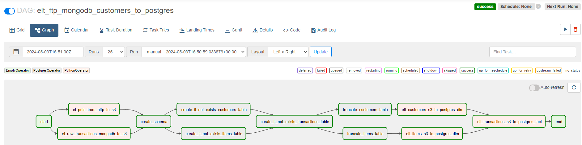
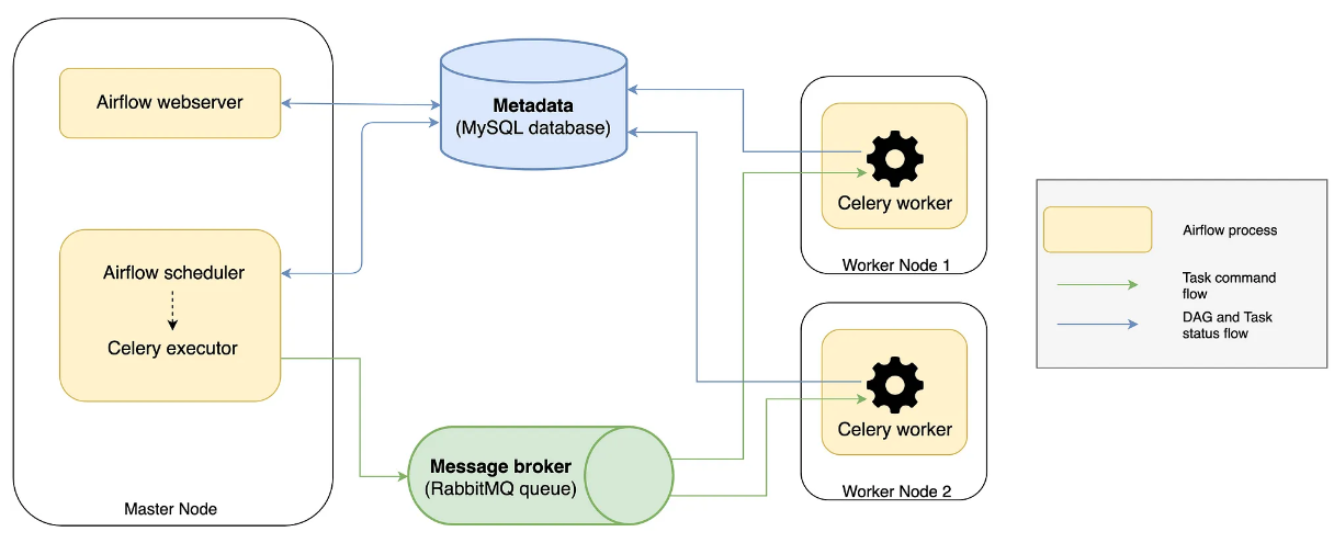
Behind the scenes, multiple worker nodes will share those tasks by using a broker pattern (ref. ), representing asynchronous messaging. Mouthful, I know, but in short, imagine a queue of tasks, each waiting to be taken by our limited resources of workers. That lovely term, scale, that you probably hear every other day? Well, that’s it. In this context, the Airflow scheduler sends the tasks to the message queue (e.g. Redis, RabbitMQ), which is later processed by workers (e.g. Celery). This processing could include, like the code above, accessing external resources, performing some calculations, and even triggering other processes. The image below represents this concept, credits to this post, wonderful resource to dive deeper.

You will see such a setup commonly when working with distributed systems, the go-to approach when dealing with massive amounts of data or processing required. Also, this concept of DAG is also used with Big Data technologies like Spark, and I encourage you to read more about it with this resource if you’re interested. Note, those concepts don’t relate only to one technology but you’ll see reused and reused as it’s more part of a paradigm or framework than an isolated feature.

Going back to our use case, let’s further explore an example of gathering the item catalogue from the transactional data. This will be part of an Airflow task that will follow the definition of the structure of the final table. We will see how we perform certain dimensional modelling techniques and transformations to get the table in tip-top form for our data scientists and analysts to explore further (e.g. price optimization).

Dimensional Modelling for Data Warehousing

Below is a task to define part of the schema of our data warehouse, specifically that of the items catalogue. We can find some typical attributes like the item’s SKU, unit price, and description. Note the presence of two attributes, DATETIME_VALID_FROM and DATETIME_VALID_TO; since the same item’s price is subject to change over time, we won’t necessarily have one row per unique item. We use those two attributes in order to identify the price that an item had over an interval of time. This concept is called Slowly Changing Dimension (or SCD) for short, and is an important concept in Dimensional Modelling. I will leave some references at the end of the articles for some more details on the different paradigms in that field, including Snowflake Schema, Star Schema, and Data Vault.

create_items_table = PostgresOperator(
        task_id="create_if_not_exists_items_table",
        postgres_conn_id=POSTGRES_CONN_ID,
        sql=f"""
        CREATE TABLE IF NOT EXISTS {POSTGRES_ITEMS_DIM_NAME} (
                ID                      VARCHAR                 ,
                STOCK_CODE              VARCHAR                 ,
                UNIT_PRICE              DECIMAL                 ,
                DESCRIPTION             VARCHAR                 ,
                DATETIME_VALID_FROM     TIMESTAMP               ,
                DATETIME_VALID_TO       TIMESTAMP               ,
                PRIMARY KEY (ID)
        );
        """,
    )

Below, we proceed with the required transformations form the JSON data that we flattened to a dataframe. We do some preprocessing like formatting dates, deduplicating, and dealing with NULLs.

After those preprocessing transformations, notice how we define the two datetime attributes mentioned above, and define a unique key to the record by hashing a combination of three attributes that could uniquely define an item at a point in time.

def etl_items_s3_to_postgres_dim():
    items_df, local_file_path = s3_to_transact_df(bucket_name=S3_TRANSACTIONS_BUCKET)
    relevant_columns = ["StockCode", "Description", "UnitPrice", "InvoiceDate"]
    items_df = items_df[relevant_columns].rename(
        {
            "StockCode": "STOCK_CODE",
            "Description": "DESCRIPTION",
            "UnitPrice": "UNIT_PRICE",
            "InvoiceDate": "INVOICE_DATE",
        },
        axis=1,
    )
    items_df["DESCRIPTION"] = items_df.groupby("STOCK_CODE")["DESCRIPTION"].transform(
        lambda x: x.ffill()
    )
    items_df["INVOICE_DATE"] = pd.to_datetime(items_df["INVOICE_DATE"])
    cols = ["STOCK_CODE", "DESCRIPTION", "UNIT_PRICE"]
    items_df["ID"] = items_df[cols].apply(
        lambda row: "|".join(row.values.astype(str)), axis=1
    )
    items_df["ID"] = items_df["ID"].apply(
        lambda x: hashlib.md5(x.encode("utf-8")).hexdigest()
    )
    items_df = items_df[
        ["ID", "STOCK_CODE", "DESCRIPTION", "UNIT_PRICE", "INVOICE_DATE"]
    ]
    items_df = (
        items_df.groupby(["ID", "STOCK_CODE", "UNIT_PRICE", "DESCRIPTION"])[
            "INVOICE_DATE"
        ]
        .min()
        .reset_index()
    )
    items_df = items_df.sort_values(["STOCK_CODE", "INVOICE_DATE"])
    items_df["DATETIME_VALID_TO"] = items_df.groupby("STOCK_CODE", group_keys=False)[
        "INVOICE_DATE"
    ].apply(lambda x: x.shift(-1).fillna(datetime(2099, 12, 31)))
    items_df["DATETIME_VALID_TO"] = items_df["DATETIME_VALID_TO"] - timedelta(seconds=1)
    items_df.rename({"INVOICE_DATE": "DATETIME_VALID_FROM"}, axis=1, inplace=True)
    postgres_sql_upload = PostgresHook(postgres_conn_id=POSTGRES_CONN_ID)
    postgres_sql_upload.insert_rows(
        schema=POSTGRES_SCHEMA_NAME, table=POSTGRES_ITEMS_DIM_NAME, rows=items_df.values
    )

Note that typically afer the preprocessing steps, we store the data in an intermediary table prior to data modelling. The resulting dimensional model is typically a view or materialized view that points to those tables. I’ve merged those steps for the sake of brevity.

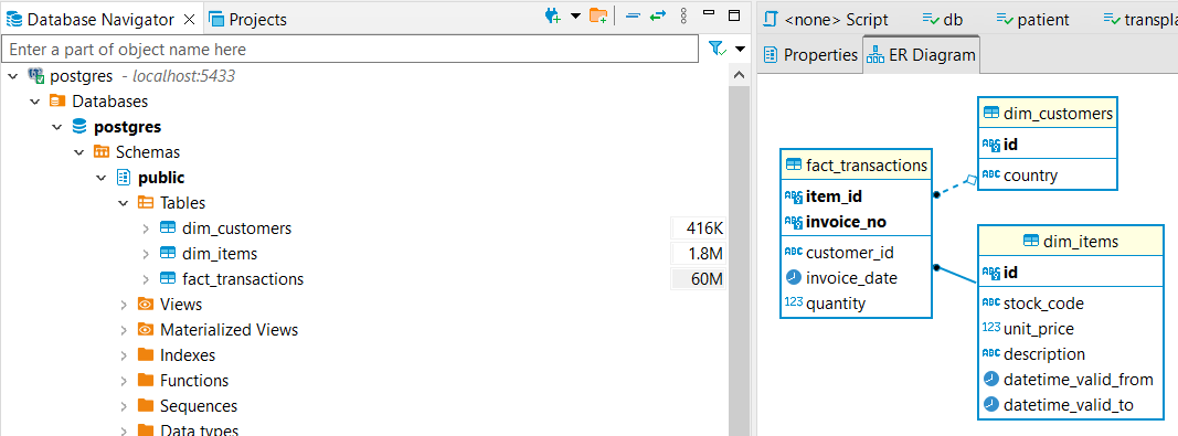
Now we see the data that our data scientists need to start developing their models.

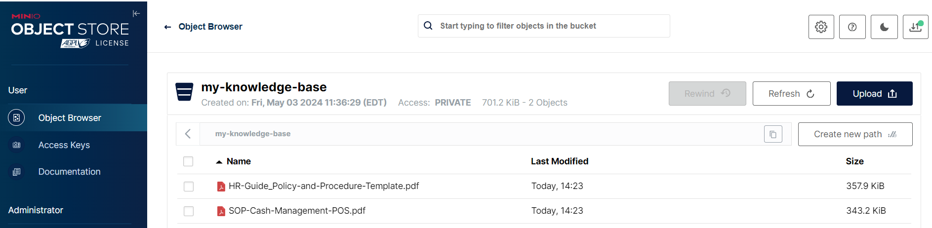
Above we see the unstructured, raw files in our data lake, which we can use to enrich our LLMs with a RAG approach. Below, the structured data model including our customers, items, and interactions between both (i.e. transactions), will be used to build models such as customer segmentation, price optimization, customer lifetime value forecasting, churn prediction, etc.

Other Considerations

With such a data architecture, we are approaching what we call a Data Fabric paradigm. However, we still need to integrate metadata management. Otherwise, how can we ensure as business users we can trust the data? We can ensure a more comprehensive data observability by including lineage and cataloguing; if we understand the journey of our data from its inception, we can maintain its integrity and trace any unexpected behavior back to its source. By integrating quality monitoring, we can help monitor and catch issues earlier on, and also use data versioning to revert to a previous working version while working on the issue, all of which can improve our SLAs.

You see, much of the life of a data engineer isn’t to just build, but much of it is to maintain. When the data changes hands so much, and something goes wrong, it’s easier to point fingers. This is why data contracts have come in place.

We could integrate those components in a future tutorial since they’re paramount at ensuring good continuity of data and build trust in the organization. Other improvements to the current project include:

1. Adding Incremental. Add logic to only get new and modified files since last ingestion to avoid duplicates. Same logic for MongoDB records. Doing a full load isn’t ideal in most cases unless for reference data.
2. Security: Add access control (RBAC possible via Airflow) and encryption for our sensitive data.

More Resources

1. Designing Data-Driven Applications by Martin Kleppmann, more conceptual but dives deep into the issues of scalability, consistency, reliability, efficiency, and maintainability.
2. The Data Warehouse Toolkit by Ralph Kimball, for dimensional modelling.
3. Data Engineering Wiki will talk about some operating models like Data Mesh, Data Fabric, and some architectures like Medallion, Kappa, Lambda, etc.