Building your AI Ecosystem Part II: Machine Learning Workflows, Packaging, and Consumption
The last part focused on how we can leverage a proper data architecture along with data pipelines and dimensional models in order to have a centralized view of your customers and operations, while keeping the data reliable and fresh.
In this part, we will focus more on the other part of the equation for AI models, which is their operationalization. We’ll also go over the interplay and dynamics between the different domains that make up an advanced analytics practice.
You have probably heard of the statistics that
- Data Scientists spend 60-80% of their time cleaning data rather than analyzing it; this comes with an opportunity cost.“Cleaning Big Data: Most Time-Consuming, Least Enjoyable Data Science Task, Survey Says” - Forbes
- As many as 87% of models don’t make it into production as VentureBeat reports.
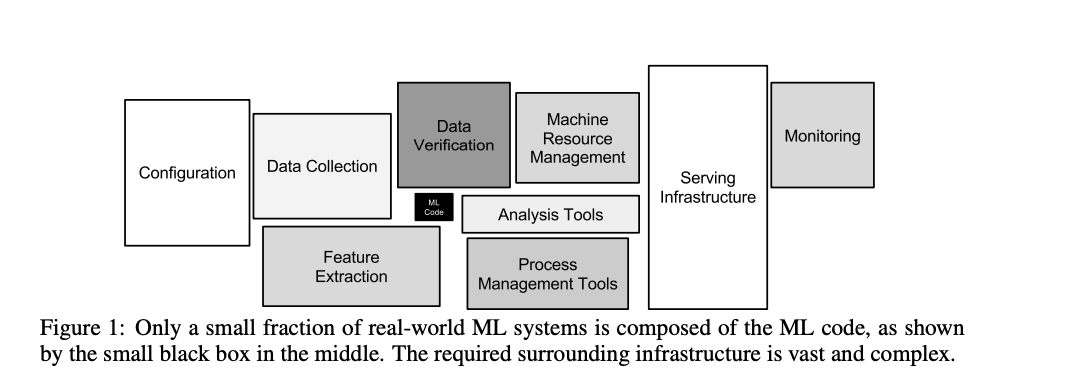
It is important to consider the multiple facets that make up a successful ecosystem for ML models to be R&D’ed in a streamlined fashion and given the ability to be maintained and trusted in prod. This is much of the concerns of MLOps, and is again more than just tools. A popularized paper, Hidden Technical Debt in Machine Learning Systems, showcased those concerns.
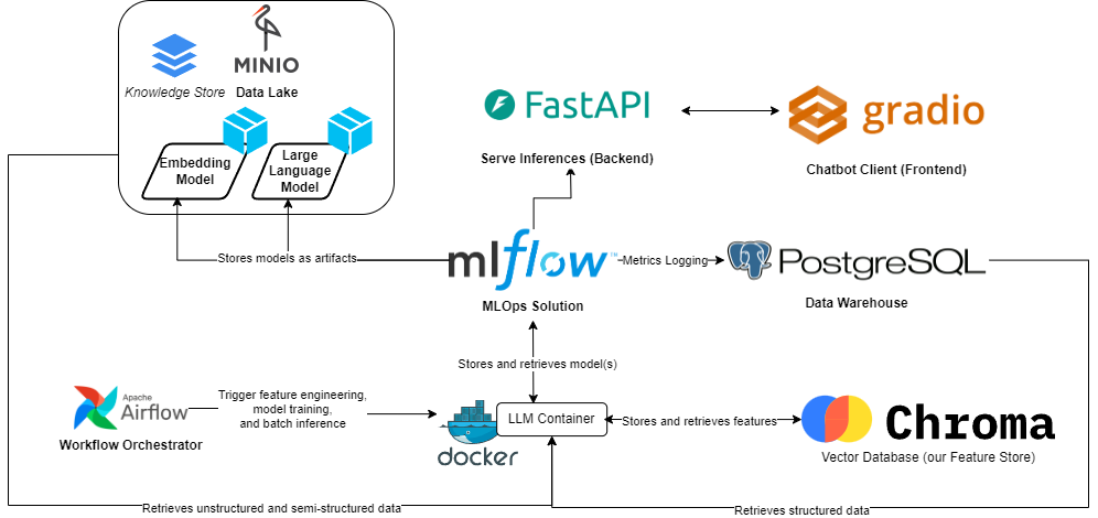
In this part as well as the series, one of our goal is to tackle those aspects. MLOps at the rescue, as it aims to answer that and goes beyond, to ensure our models are resilient and reliable. A target architecture can look like the following, going over the integration of a Retrieval Augmented Generation, (or RAG)-based LLM as an example.
Model Development & Experimentation
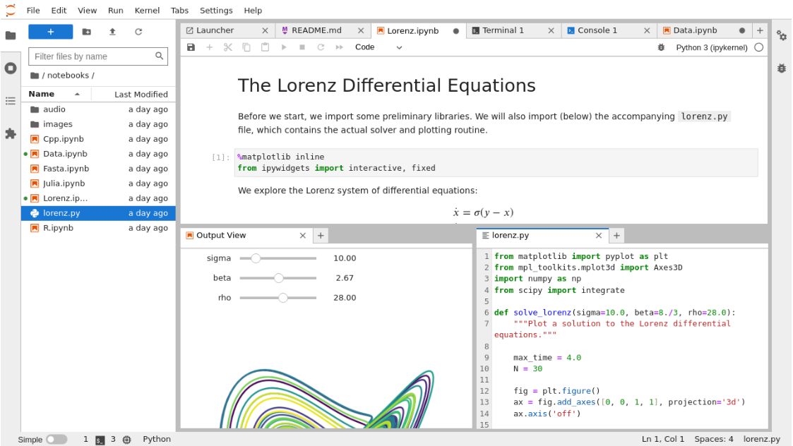
In the typical experimentation of a data scientist (DS), they dive into their experiments in a sandbox environment such as an interactive python notebook (.ipynb), whether through Jupyter Notebooks, Microsoft ML Studio, AWS SageMaker, Google Colab, etc. In the previous part, Data Engineers centralized the data needed for DS models, including a knowledge base in the data lake and tabular data in the data warehouse, facilitating easy data discovery and extraction.
The provided data is clean and formatted, allowing the DS to proceed with Data Wrangling, including Exploratory Data Analysis, Feature Engineering, Modelling, etc. Here is an example fo how such workspace can look like.
Moving forward, let’s assume the DS has engineered relevant features, such as semantic representations of data from the knowledge base. Additionally, they have found, trained, and fine-tuned an LLM that enriches responses to user queries. In the next part of the series, we’ll delve into the detailed DS process, including considerations at each step leading to this outcome. For now, let’s consider the model found is TheBloke–Llama-2-7b-Chat-GGUF, a pre-trained model from HuggingFace, evaluated and fine-tuned with hyper-parameters {"temperature": 0.75, "top_p": 1, "n_ctx": 4096, "max_tokens": 4096, "top_k": 4, "chain_type": "stuff"}.
While impressive, the demo presented by the DS is limited to their workspace, whether local or cloud-based. The crucial next step is to transition the model into production and, more importantly, ensure its continuous maintenance and improvement.
Model Integration
To do so, the ML Engineer will come into the picture, and will will be responsible of taking the source code from the sandbox environment, potentially bonify it, and structure it in a way that we are able to have some automated pipelines that could automate the feature engineering, model training, and inference steps.
Now, the issue is, while it looks enticing to simply put the code as tasks to be ran by the scheduler, we are still missing a key aspect that makes most if not all data scientists and ML engineers alike to pull their hair; system environment configuration and dependency management. Without the right library versions and system specifications, we cannot guarantee that the model will run and work as expected.
Model Packaging
To solve this, a common pattern is encapsulating the AI-related logic in a docker image that contains the necessary source code and setup for that, e.g. downloading the necessary binaries, drivers for interfacing with the GPU of the host machine etc. as well as the library dependencies. Below, we can see part of that setup via the Dockerfile.
FROM nvidia/cuda:12.3.1-devel-ubuntu20.04

# Install Python
RUN apt-get update && DEBIAN_FRONTEND=noninteractive \
    apt-get install -y software-properties-common && \
    DEBIAN_FRONTEND=noninteractive add-apt-repository -y ppa:deadsnakes/ppa && \
    apt-get install -y python3.10 curl && \
    curl -sS https://bootstrap.pypa.io/get-pip.py | python3.10

RUN curl -sSL https://install.python-poetry.org | python3.10 - --preview
RUN pip3 install --upgrade requests
RUN ln -fs /usr/bin/python3.10 /usr/bin/python

# LLM specific binaries
RUN apt-get update && \
    apt-get install -y build-essential && \
    apt-get install -y libgl1 && \
    apt-get install -y poppler-utils && \
    apt install -y libpython3.10-dev &&\
    apt install -y python3.10-distutils && \
    apt-get install -y libcairo2-dev pkg-config python3-dev && \
    apt-get install -y libtesseract-dev && \
    apt-get install -y tesseract-ocr


WORKDIR /app

COPY requirements.txt .

ENV CMAKE_ARGS="-DLLAMA_CUBLAS=ON"
RUN python -m pip install --no-cache-dir -r requirements.txt

COPY . .

CMD ["/bin/bash"]
This docker image is executable, is packaged and versioned, and fits nicely in a CI/CD pipeline. It will spawn a terminal based command line, where we can encapsulate the instructions related to feature engineering, model training, and model inference. As we can see in our architectural diagram above, it will be quite the literal brain of our system. Feel free to navigate to the src/terminal.py file of the project to observe the parsing logic for the terminal command line, and how it triggers the required functionality mentioned above via the model_handler and data_handler.
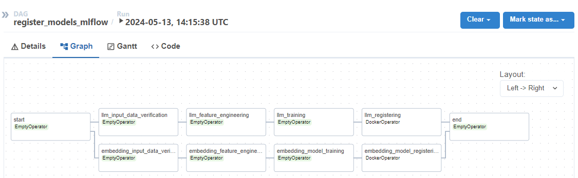
Model Pipelines
Now those pieces can be fit into a workflow orchestrator, where we can automate steps like the following:
-
Feature Storage: We automate the extraction of the knowledge base from our data lake,
MinIO, the embeddings computations done by the Data Scientists, and their storage in our Feature Store, in our case a vector storage calledChromaDBthat will allow us to later retrieve them during inference. -
Model Registering: We automate the model selection, training, and fine-tuning of our models, as well as their packaging into artifacts that could be more seamlessly loaded and used given we have the right environment for it.
Let us dive a bit more into thoe pipelines as well as the underlying technologie and their importance.
Feature Store
In this part, we encapsulate the data extraction, validation, and preparation code. The feature store isn’t only used for the model integration but also for aiding the data scientist’s development. Without a feature store, other data scientists wouldn’t be able to share their often-times common data transformations, as well as open the door to having a different logic of feature engineering in training vs. inference. With redundancy comes extra time that could’ve been spent elsewhere, as well as the potential of introducing bugs and overall having a more failable and less resilient system.
We will enrich the data pipeline we developed in last part to adding a task that will ingest our raw data from the knowledge base, and transform it in a way that could ultimately help us enrich our LLM’s predictions.
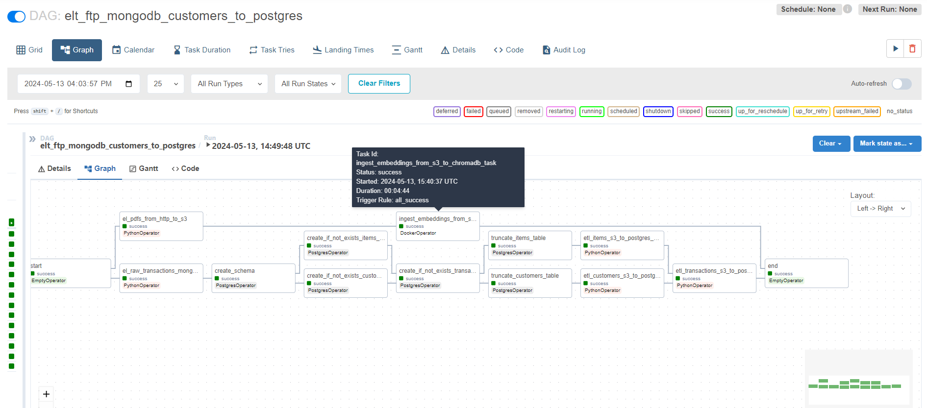
The feature engineering logic is triggered by the workflow orchestrator via a command as follows. We ensure those pipelines are configurable, and we pass the approrpaite connection strings (encrypted), and the user roles could be validated (RBAC) in a centralized manner.
 ingest_embeddings_from_s3_to_chromadb_task = DockerOperator(
        task_id="ingest_embeddings_from_s3_to_chromadb_task",
        image="{{ params.docker_image_name }}",
        command=[
            "sh",
            "-c",
            """
        cd src && \

        python -m terminal ingest_data_from_mode \
        --mlflow_tracking_uri http://{{ var.value.mlflow_host }}:{{ var.value.mlflow_port }} \
        --mlflow_registry_uri {{ json.loads(conn.minio.extra)['endpoint_url'] }} \
        --embedding_model_uri "{{ params.embedding_model_uri }}"  \
        --chroma_host {{ var.value.chroma_host }} \
        --chroma_port {{ var.value.chroma_port }} \
        --chroma_collection_name "{{ params.chroma_collection_name }}" \
        --embeddings_model_source mlflow \
        --minio_access_key {{ json.loads(conn.minio.extra)['aws_access_key_id'] }} \
        --minio_secret_key {{ json.loads(conn.minio.extra)['aws_secret_access_key'] }} \
        --minio_bucket_name "{{ params.minio_bucket_name }}" \
        --data_source minio \
        --full

    """,
        ],
        device_requests=[docker.types.DeviceRequest(count=-1, capabilities=[["gpu"]])],
        dag=dag,
        network_mode="container:llm"
    )
Feature stores come in various forms, commonly sourcing inputs from the data warehouse and also storing them there. In the example we’re discussing, it’s common to utilize a model for feature engineering, especially in tasks involving computer vision and NLP. In other tutorials, we’ll explore additional examples, such as dealing with tabular data. For instance, in customer analytics, typical features include Recency, Frequency, and Monetary value (RFM for short) for each customer. These features serve as inputs to numerous models, including churn and lifetime value prediction.
Model Registry
Just like the feature store, the model registry isn’t only helpful for model integration but helps the data scientist in their R&D, by helping keep track of their experiments so they can easily compare them and roll back to them in case they don’t find any improvements. It is a sort of version control.
When it comes to integration, this centralized version control can also be useful when it comes to auditing or rolling back to a previous working version in case of errors in production, while a fix is being worked on. Note in this case, for the rolling back to work we also need to have a version control for our data, but this is outside the scope of this part of the series.
In our workflow orchestrator, we can develop a pipeline to replicate the logic of the experiment, and add a couple of layers of data verification and model serialization.
-
Step 1. Data Verification: we validate the quality of the training data, including its completeness (NULL values) and format (proper data type and range of values).
-
Step 2. Feature Engineering: we gather some features from the feature store and potentially compute some on the same machine.
-
Step 3. Model Selection & Fine-Tuning; here is an example of this step from a prior project I’ve worked on.
# test these hyperparameters to save
penalizer_coefs = [0, 0.01, 0.1, 1]
models_dict = {}
for model_class in [BG_NBD, Pareto_NBD]:
    model_str = model_class.__name__.split(".")[-1]
    models_dict[model_str] = []
    for penalizer_coef in penalizer_coefs:
        try:
            model = model_class(penalizer_coef=penalizer_coef)
            model.fit(rfm_matrix=train_rfm_table)
            evaluation_df = model.evaluate(
                test_rfm_tb=test_rfm_table, train_rfm_tb=train_rfm_table
            ).dropna()
            evaluation_df = winsorize_df(
                df=evaluation_df, col="Actual", cutoff=0.02
            )
            predictions = evaluation_df["Expected"].to_numpy()
            targets = evaluation_df["Actual"].to_numpy()
            models_dict[model_str].append(
                {
                    "penalizer_coef": penalizer_coef,
                    "performance": calc_performance(targets, predictions),
                    "model": model,
                }
            )
        except Exception:
            print(traceback.format_exc())
# Find the item with the minimum RMSE value across all models
min_item = min(
    (item for sublist in models_dict.values() for item in sublist),
    key=lambda x: x["performance"]["rmse"],
)
# Extract the value of the 'model' key from the item with minimum RMSE
best_model = min_item["model"]
best_model_fully_trained = best_model.__class__()
best_model_fully_trained.fit(rfm_matrix=rfm_table)
best_model_key = best_model.__class__.__name__.split(".")[-1]
with open(f"{best_model_key}.dill", "wb") as fp:
    dill.dump(best_model_fully_trained, fp)
In this project however, we simply need retrieve the weights of our embedding model and LLM from HuggingFace.
- Step 4. Produce the Artifacts: we serialize the model by converting the model object (which includes the weights and hyper-parameters) into bytes. We encapsulate the logic of model de-serialization, loading, data validation, and inference. We take all this, in addition to the model dependencies, and register them. All this is so that we can easily make use of the model during inference. Those will be stored as artifacts in our data lake.
We are leveraging a popular MLOps tool called MLFlow that will help us do that, and abstracts the logic of the final steps quite seamlessly:
log_model(
    artifact_path="model",
    python_model=LLMWrapper(),
    artifacts=artifacts,
    signature=ModelSignature(
        inputs=Schema(
            [
                ColSpec(type="string", name="input_text"),
            ]
        ),
        outputs=Schema([ColSpec(type="string", name="result")]),
    ),
    input_example={
        "input_text": "How many sales have we made in the past year in the UK?"
    },
    conda_env=conda_spec_path,
    model_config=model_config
)
You could see the logic of the model wrapping under src/model_handler.py and src/llm_embedding_pipeline.py.
This model training, fine-tuning, and registration is part of a pipeline that will be scheduled or triggered based on an event.
After running the pipeline in our orchestrator, we can observe some metadata about the model run as well as the saved artifacts, and we can then version and register it.
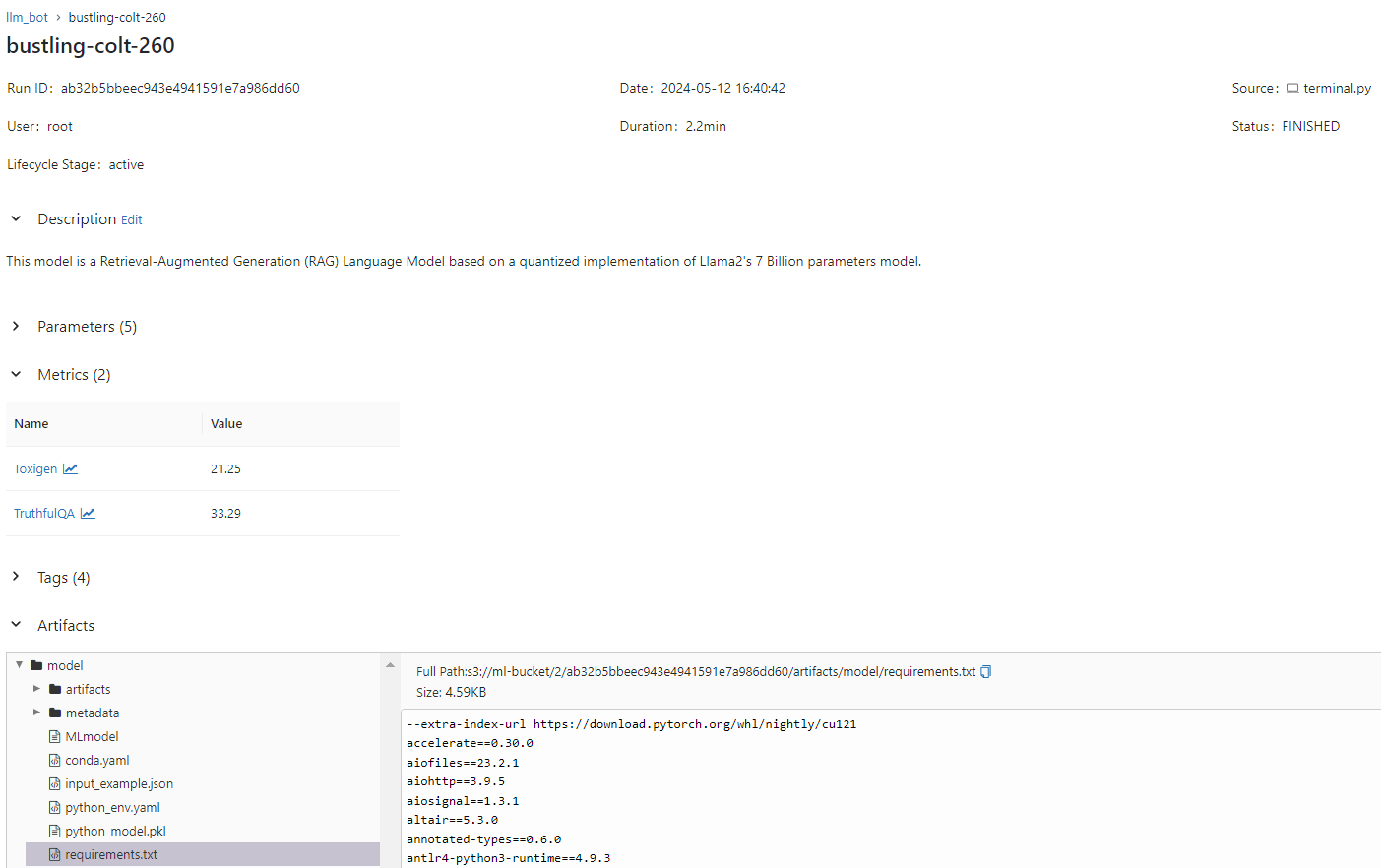
As we can see, in this way we can track experiments as well as the models to be used in production, and forms a key part of reproducibility.
Model Consumption
In the final section, we will see how we can actually make use of those models as an end product. Typically, the models could be utilized in two ways: real-time or batch.
Batch Mode
Models can be integrated into a pipeline to make predictions in bulk. In this setup, data is collected and processed in batches, and predictions are made on entire datasets (e.g. full mode) or subsets (e.g. incremental mode).
This could be useful in the case of dealing with large amounts of data or when time sensitivity is less critical e.g. customer segmentation, predictive maintenance…
In the case of a RAG, I skipped a detail for the feature engineering part; the embeddings generated and stored in our vector store are actually done by an embedding model. This is an example of a batch based predictions where we take our knowledge base every so often (e.g. weekly), and can appropriately create, update, or delete the required embeddings.
Real-Time Mode
In this scenario, the models are loaded onto a server equipped with the necessary environment. This server exposes an API endpoint to serve predictions, typically on one or a few data points at a time.
This approach is beneficial in the cases of live user interactions (e.g. recommendation engines, chatbots…) or real-time monitoring systems (e.g. anomaly detection, sentiment analysis…), either way when immediate responses are required.
In our case, we feed the LLM in a server with FastAPI, where we install the appropriate dependencies from the artifacts stored by MLFlow in our data lake. We then load the model at startup
from fastapi import FastAPI
from model_handler import LLMLoader
from data_handler import EmbeddingLoader
from langchain.callbacks.manager import CallbackManager
from langchain.callbacks import StreamingStdOutCallbackHandler
from constants import *

app = FastAPI()

# Set up callback manager
callback_manager = CallbackManager([StreamingStdOutCallbackHandler()])
# Load embedding model
embedding_model = EmbeddingLoader().load_from_mlflow(model_name=EMBEDDING_MODEL_NAME)
# Load LLMLoader
qa = LLMLoader().load_from_mlflow(
    embedding_model=embedding_model,
    chroma_host=CHROMA_DB_HOST,
    chroma_port=CHROMA_DB_PORT,
    collection_name=CHROMA_DB_COLLECTION,
    model_id=MODEL_ID,
    model_basename=MODEL_BASENAME,
    context_window_size=CONTEXT_WINDOW_SIZE,
    n_gpu_layers=N_GPU_LAYERS,
    n_batch=N_BATCH,
    max_new_tokens=MAX_NEW_TOKENS,
    cpu_percentage=CPU_PERCENTAGE,
    use_memory=USE_MEMORY,
    system_prompt=SYSTEM_PROMPT,
    chain_type=CHAIN_TYPE,
    model_type=MODEL_TYPE,
    callback_manager=callback_manager,
)


@app.get("/answer/")
async def answer(question: str):
    print("Received Question!\n", question)
    res = qa(question)
    answer, docs = res["result"], res["source_documents"]
    if len(docs):
        s = "\n\nHere are the relevant sources for this information:\n"
        unique_sources = list(set([doc.metadata["source"] for doc in docs]))
        for i, doc in enumerate(unique_sources):
            s += f"• {doc}\n"

        answer = f"{answer}{s}"

    return {"response": answer}


if __name__ == "__main__":
    import uvicorn

    uvicorn.run(app, host="0.0.0.0", port=6060)
We can then interact with our chatbot:
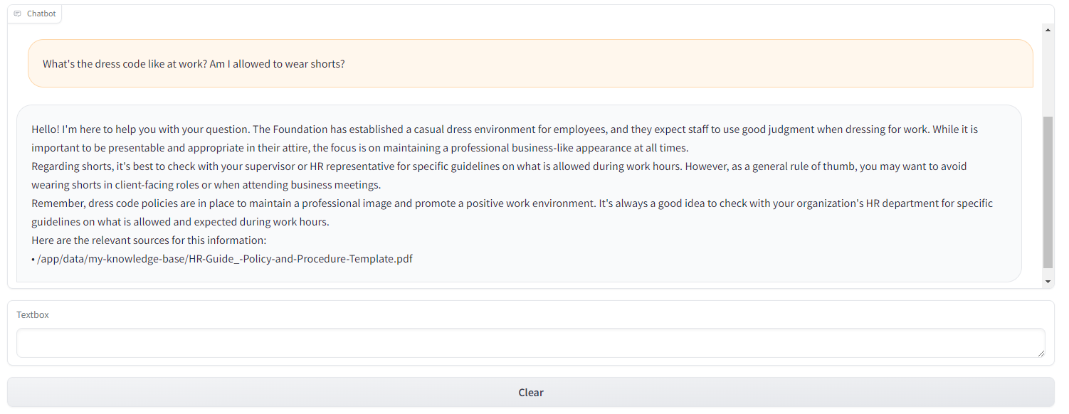
In conclusion, whether real-time or batch, those model predictions can be fed downstream into dashboards or applications. The batch predictions are stored in the data warehouse and queried from there, whereas the real-time ones could be done via APIs (e.g. Flask, Django, FastAPI) or in streaming fashion (Apache Kafka or Apache Pulsar) for higher throughput.
Closing Notes
As we revisited the concept of workflow orchestration from Part I, we begin to notice the interplay of roles within this domain. Let’s conceptualize a simplified workflow to illustrate this:
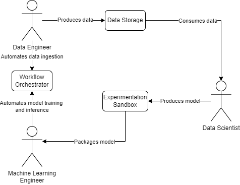
Decoupling is paramount. According to Gene Kim et al., in their book “Accelerate”, “high performance [in software delivery] is possible with all kinds of systems, provided that systems—and the teams that build and maintain them — are loosely coupled. This key architectural property enables teams to easily test and deploy individual components or services even as the organization and the number of systems it operates grow—that is, it allows organizations to increase their productivity as they scale.”
This tutorial assumed that our Data Scientist has already built the model. Part I and Part II focused on the processes of a Data Engineer and an ML Engineer, respectively, and how they could interface together and with a Data Scientist. In the next part, we will delve into more detail on the Data Scientist’s process, including the considerations they take in exploratory data analysis, feature engineering, model selection, fine-tuning, etc. Finally, in the last part, we will discuss observability, re-training strategies, and other aspects vital for maintaining a robust AI ecosystem.